5.5.1. Backtracking¶

Backtracking is a method, which allows us to systematically visit all possible combinations (solutions). It is a “brute-force” algorithm, whose implementation is typically straightforward. The method is useful when the number of combinations is so small that we have time to go through them all. In this chapter, we will first familiarize ourselves with the backtracking algorithms, which go through combinations of numbers. After this, we will see how you can use the backtracking in two problems and how to make the search for optimal solution more efficient.

5.5.2. From loops to recursion¶

Suppose we want to go through all combinations of 𝑛 numbers, where each number is an integer between \(1...m\). There are a total of \(m^n\) such combinations (there are \(n\) points and in each point the number can be chosen in \(m\) ways). For example, if \(n=3\) and \(m=4\), the combinations are \([1,1,1], [1,1,2], [1,1,3], [1,1,4], [1,2,1], [1,2,2], [1,2,3], [1,2,4]\), etc.

If the value of \(n\) is known in advance, we can create \(n\) nested loops, each of which goes through \(m\) numbers. For example, the following code loops through all combinations in case \(n=3\)\(n=3\)

for a in range(m):
    for b in range(m):
        for c in range(m):
            print(a, b, c) 

This is a good solution in itself, but there is one problem: the value of \(n\) affects on the number of loops. If we wanted to change the value of \(n\), we would have to change the amount of loops in the code, which is not practicable. However, we can implement a solution recursively using backtracking so that the same code works for all values of \(n\).

5.5.3. Implementing the search¶

The following recursive procedure search forms combinations using backtracking. This can be used as brute-force search to find the optimal solution. The parameter \(k\) is the position in the array where the next number is placed. If \(k=n\) some combination has been completed, in which case it is printed. Otherwise, the search goes through all the ways to place numbers \(1...m\) in position \(k\) and continues recursively to \(k+1\). The search starts with the call search(0), and numbers is an \(n\)-sized array in which the combination is formed.

def search(k):
    if k == n:
        print(numbers)
    else:
        for i in range(1, m + 1):
            numbers[k] = i
            search(k + 1)

Figure 5.5.1 shows how the search starts in case 𝑛=3 and \(m=4\). The sign “\(-\)” means a number that has not been selected yet. The first level of the search selects the combination to position \(0\) of the first number. There are four options for choosing this, since the possible numbers are \(1...4\), so the search branches into four parts. After this, the search continues recursively and selects the numbers for the other positions.

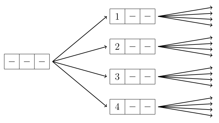
Figure 5.5.1: Forming the combination \(n=3\) and \(m=4\).¶

We can evaluate the efficiency of the algorithm by calculating how many times the search procedure is called in total during the search. The procedure is called once with parameter \(0\), \(m\) times with parameter \(1\), \(m^2\) times with parameter \(2\), etc., so the number of invitations is total

At the last level of recursion, more invitations are made than at all other levels combined.

5.5.4. Subsets¶

Let us then examine the situation, where we want to go through all subsets of a set with \(n\) elements. There are a total of \(2n\) subsets, because each element either belongs or does not belong to a subset. For example, \(\{2,5\}\) and :math`{3,5,9}` are subsets of the set \(\{2,3,5,9\}\). It turns out that we can form subsets by going through all combinations of \(n\) numbers, where each number is \(0\) or \(1\). The idea is that each number in the combination tells whether a certain element belongs to a subset. For example, when the set is \(\{2,3,5,9\}\), the combination \([1,0,1,0]\) matches subsets \(\{2,5\}\) and the combination \([0,1,1,1\)] corresponds to the subset \(\{3,5,9\}\).

The following pseude code shows how we can visit all subsets using backtracking. The procedure search chooses, whether the element in \(k\) is included in the subset or not, and marks this information in the array choice. As before, the search starts with the call search(0).

def search(k):
    if k == n:
        # process the subset
    else:
        for i in (0, 1):
            choice[k] = i
            search(k + 1)

5.5.5. Permutations¶

With backtracking, we can also loop through all permutations, i.e. different orders of elements. When there are \(n\) elements in the set, in total \(n!\) permutations can be formed. For example, \(\{2,4,1,3\}\) and \(\{4,3,1,2\}\) are permutations of the set \(\{1,2,3,4\}\).

In this situation, we want to go through combinations of \(n\) numbers, where each number is between \(1...n\) and no number is repeated. We achieve this by adding a new array named included which tells if a certain number is already included. At each step, the search selects only such numbers for the combination which have not been selected before.

def search(k):
    if k == n:
        # process permutation
    else:
        for i in range(1, n + 1):
            if not included[i]:
                included[i] = True
                numbers[k] = i
                search(k + 1)
                included[i] = False

5.5.6. The N Queens Problem¶

Next, we will go through two more demanding examples on how to utilize the backtracking to solve problems.

Our task is to calculate, in how many ways \(n\) queens can be placed on an \(n \times n\) chessboard so that no two queens threaten each other. In chess, queens can threaten each other horizontally, vertically or diagonally. For example, in the case of \(n=4\), there are two possible ways to place the queens as shown in Figure 5.5.2.

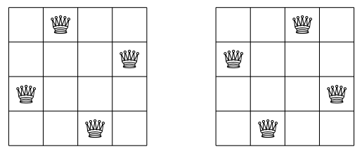
Figure 5.5.2: Solution to the queens problem with \(n=4\).¶

We can solve the task by implementing an algorithm, which goes through the board from top to bottom and places one queen for each row. Figure 5.5.3 shows the operation of the search in the case \(n=4\). The queen of the first row can be placed in any column, but in the following lines, previous selections limit the search. The figure shows the placement of the second queen, when the first queen is in the second column. In this case, the only option is that the second queen is in the last column, because in all other cases the queens would threaten each other.

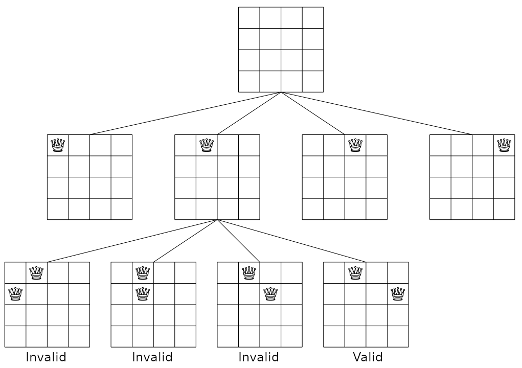
Figure 5.5.3: Applying backtracking to the \(n\) queens problem.¶

The following function search presents the backtracking algorithm which calculates the solutions to the \(n\) queens problem:

def search(y):
    if y == n:
        counter += 1
    else:
        for x in range(n):
            if can_be_placed(y, x):
                location[y] = x
                search(y + 1)

We assume that the rows and columns of the board are numbered from \(0...n-1\). The parameter \(y\) tells on which row the next queen should be placed, and the search starts with the call search(0). If the row is \(n\), all queens have already been placed, so one solution has been found. Otherwise, a loop that goes through the possible columns (\(x\)) is executed. If the queen can be placed in the column \(x\) i.e. it does not threaten any previously placed queen, the table location is updated accordingly (the queen \(y\) is in the column \(x\)) and the search continues recursively. The function can_be_placed examines whether a new queen can be placed on row \(y\) and column \(x\).

Now we have an algorithm that allows us to review solutions to the queen problem. The algorithm solves cases with small values of \(n\) very fast, but with larger values of \(n\), the algorithm starts to take a lot of time. The reason for this is that the number of locations where the queens can be placed increases exponentially. For example, in the case of \(n=20\), there are already more than 39 billion different solutions.

However, we can try to speed up the algorithm by improving it its implementation. One easy boost is to take advantage of symmetry. Each solution to the queen problem is matched by another solution, which is obtained by mirroring the solution horizontally. For example, in Figure 5.5.2, the solutions can be changed to each other by mirroring. Thanks to this observation, we can halve the execution time of the algorithm adding the requirement that the first queen must be placed to the left half of the board, and finally multiplying the answer by two.

However, the queen problem is fundamentally a hard problem, and no essentially better solution than brute force is known. Currently, the largest case with a known solution is \(n=27\). Processing this case took about a year with a large computing cluster.

5.5.7. Allocating tasks¶

Let’s consider a situation where there are \(n\) tasks and \(n\) employees. Tasks should be distributed to the employees so that, each employee performs exactly one task. For each task-employee combination the cost for completing the task is known. The goal is to find a solution where the total cost is as low as possible. A table below shows an example case where \(n=3\). The optimal way to divide the tasks is that Employee B performs the first task, C performs second task, and A performs the third task. The total cost of this solution is \(1+2+5=8\).

We assume that tasks and employees are numbered from \(0...n-1\) and we can read from the table array cost[a][b] how much does the task \(a\) costs when performed by the employee \(b\) We can implement a backtracking algorithm which goes through the tasks in order and chooses an employee for each. The following procedure search takes two parameters: \(k\) is the task to be processed next and \(h\) is the cost so far. The search starts with the call search(0,0). The table included keeps track of which employees have already been given a task, and the variable \(p\) is the total cost in the best solution found so far. Before the search, the value of the variable \(p\) is set to \(\infty\) because no solution exists yet.

def search(k, h):
    if k == n:
        p = min(p, h)
    else:
        for i in range(n):
            if not included[i]:
                included[i] = True
                search(k + 1, h + cost[k][i])
                included[i] = False

This is a working backtracking algorithm, and at the end of the search, the variable \(p\) has the total cost of the best solution. However, the algorithm is very slow because it always goes through all the \(n!\) possible solutions. Since we only want to find the best solution and not go through all the solutions, we can improve the algorithm by adding a condition which stops forming a solution if it cannot get better than an earlier solution.

5.5.8. Branch And Bound¶

We next test the previous algorithm with the case, where \(n=20\) and the table cost contains random integers between \(1\) and \(100\). In this case, the algorithm described above would go through

different solutions which would take hundreds of years. In order to solve the case, we need to improve the algorithm so, that it does not go through all solutions but still finds the best solution. This is where a technique called branch and bound can be applied. The idea is to make the backtracking more efficient by reducing the number of solutions to be investigated with suitable upper and lower bounds.

The key observation is that we can restrict the search with the help of the variable \(p\). This variable has at every moment the total cost of the best solution found so far. Therefore it tells the upper bound on how large the total cost of best solution can be. On the other hand, the variable \(h\) has the current cost of solution being formed. This is the lower bound for the total cost. If \(h>=p\) the solution being formed cannot get better than the earlier best. We can add to the following inspection to the beginning of the algorithm:

def search(k, h):
    if h >= p:
        return
    ...

Thanks to this, the formation of the solution ends immediately if its cost is equal to or higher than the cost of the best known solution. With this simple modification the problem (\(n=20\)) can be solved within minutes instead of hundreds of years.

We can improve the algorithm even more by calculating a more accurate estimate for the lower bound. The cost of the solution under construction is certainly at least \(h\) but we can also estimate how much employees allocated for the remaining tasks add to the cost:

Here the function estimate should give some estimate on how much does it cost to complete the remaining tasks \(k...n-1\). One simple way to get an estimate is to go through the remaining tasks and choose the cheapest employee for each task without caring whether the employee has been selected before. This gives the lower bound for the remaining costs. With this modification the original problem can be solved in seconds.

This page was translated and modified from Antti Laaksonen, Tietorakenteet ja algoritmit (Chapter 8) published under Creative Commons BY-NC-SA 4.0 license.